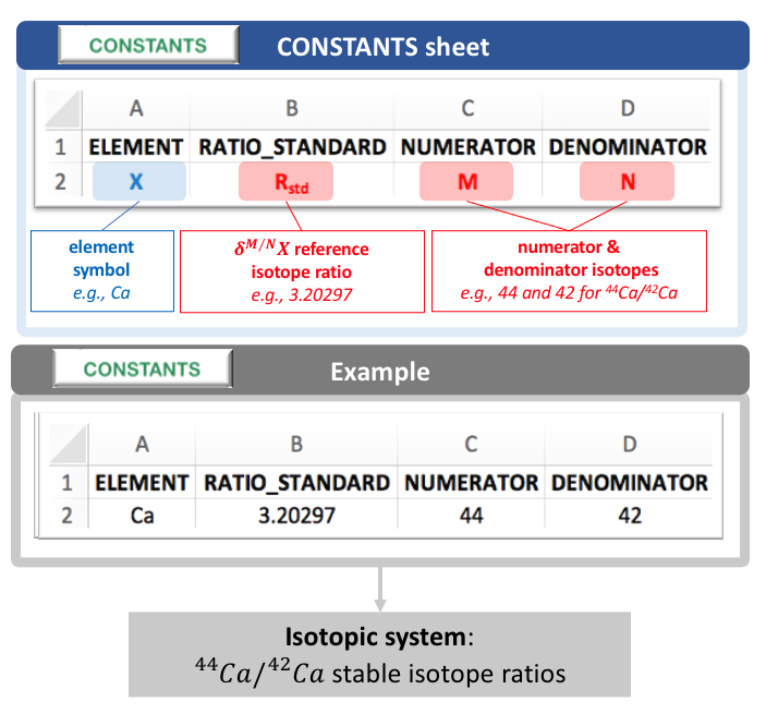
4 Main arguments and outputs
The run_isobxr function takes required and optional
arguments that are described in this section.
All arguments definitions of the run_isobxr function are
accessible in its documentation called as follows:
?run_isobxr4.1 Required arguments
The arguments required to run the run_isobxr function
are exemplified and described here with the first tutorial example (see
tutorial here):
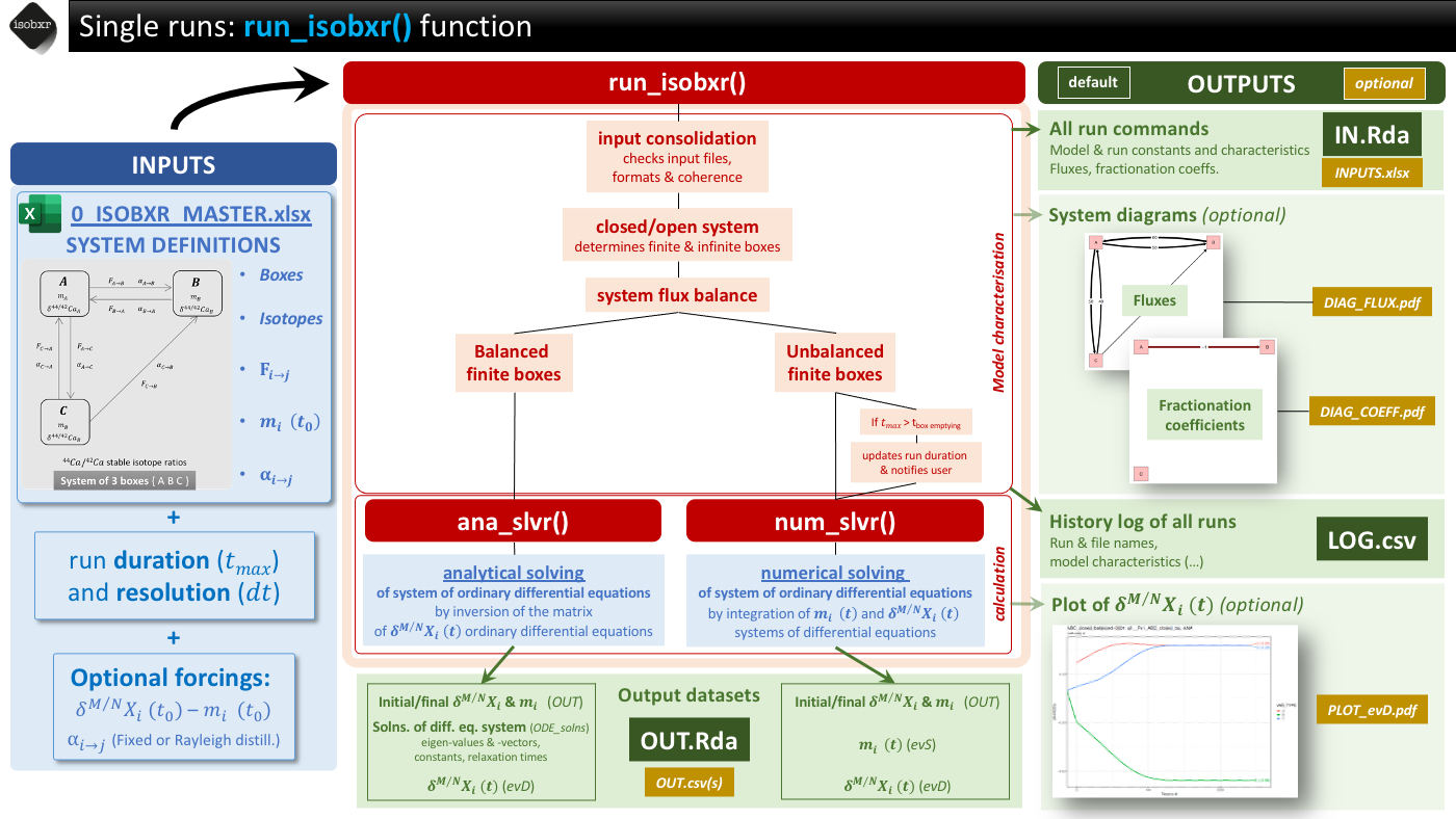
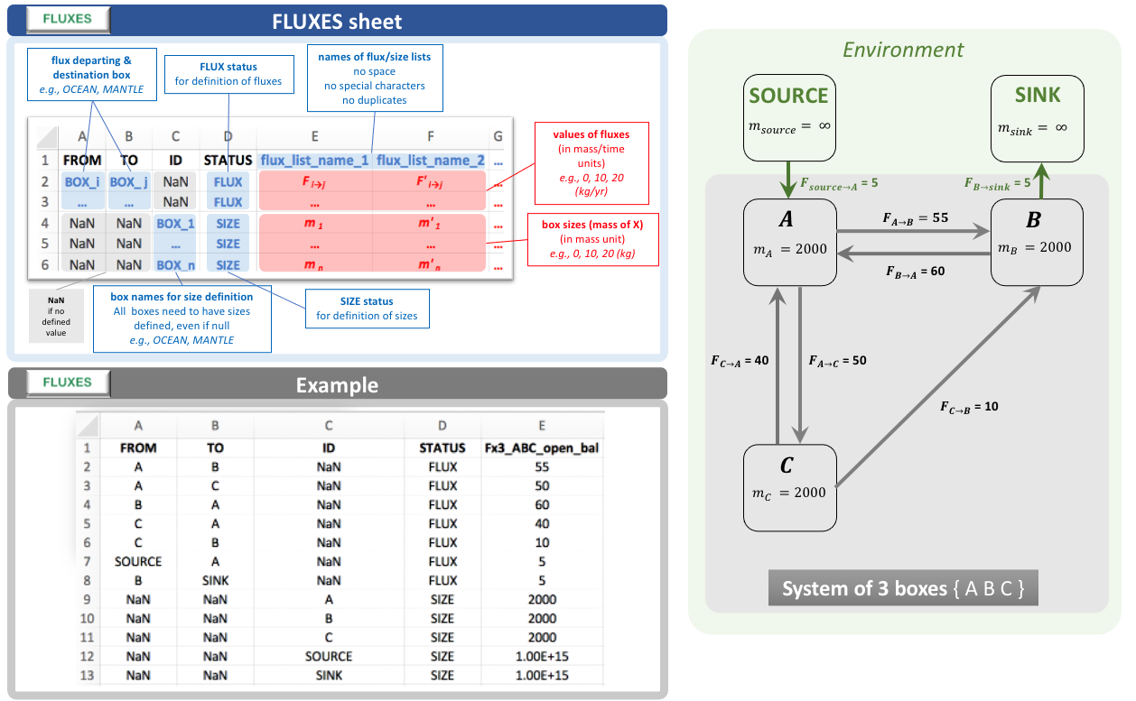
run_isobxr(workdir = "/Users/username/Documents/1_ABC_tutorial",
           SERIES_ID = "ABC_closed_balanced", # defining the name of the SERIES of run
           flux_list_name = "Fx1_ABC_closed_bal", # calling the list of fluxes
           coeff_list_name = "a1", #  calling the list of coefficients
           t_lim = 2500, # running model for 1000 time units
           nb_steps = 250, # running model with 100 steps
time_units = c("d", "yr")) # plot results in years as time units.- workdir
- Working directory of 0_ISOBXR_MASTER.xlsx master file and where output files will be stored if saved by user (save_run_outputs = TRUE, default is FALSE).
- SERIES_ID
- Name of the model series the run belongs to. It determines the folder in which the output files will be stored if saved by user (save_run_outputs = TRUE, default is FALSE).
- flux_list_name
- Name of the list of fluxes and initial box sizes to be used for the run, calling (by its header name) a single column of the FLUXES sheet of the 0_ISOBXR_MASTER.xlsx file.
- coeff_list_name
- Name of the list of fractionation coefficients to be used for the run, calling (by its header name) a single column of the COEFFS sheet of the 0_ISOBXR_MASTER.xlsx file.
- t_lim
- Run duration, given in the same time units as the fluxes.
- nb_steps
- Number of calculation steps. It determines the resolution of the run.
- time_units
-
- Vector defining the initial time unit (identical to unit used in fluxes), followed by the time unit used for the graphical output
- to be selected amongst the following: micros, ms, s, min, h, d, wk, mo, yr, kyr, Myr, Gyr
- e.g., c(“d”, “yr”) to convert days into years
4.2 Default and optional outputs
By default, the run_isobxr prints a summary plot of the
run outputs (evolution of delta values and box sizes) in the R
session.
All run_isobxr output data is stored in a temporary
directory by default.
The user can save these outputs to their working directory by changing the save_run_outputs argument to TRUE.
The run_isobxr outputs are structured as follows:
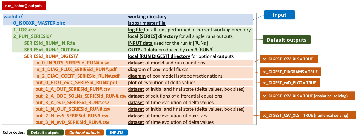
In addition to the default outputs, the run_isobxr
function allows to:
- export system diagrams (as pdf, using to_DIGEST_DIAGRAMS = TRUE)
- export evolution of delta values (as pdf, using to_DIGEST_evD_PLOT = TRUE)
- export input and output data (as csv and xlsx, using to_DIGEST_CSV_XLS = TRUE)
These arguments are called as follows (using example used in tutorial):
run_isobxr(workdir = "/Users/username/Documents/1_ABC_tutorial",
           SERIES_ID = "ABC_closed_balanced",
           flux_list_name = "Fx1_ABC_closed_bal",
           coeff_list_name = "a1",
           t_lim = 2500,
           nb_steps = 250,
           time_units = c("d", "yr"),
           to_DIGEST_DIAGRAMS = TRUE, # default is TRUE
           to_DIGEST_evD_PLOT = TRUE, # default is TRUE
           to_DIGEST_CSV_XLS = TRUE  # default is FALSE
)- Note
-
All
run_isobxroutputs are not saved by default. Set save_run_outputs = TRUE to save outputs to a local working directory.
4.3 Additional forcing arguments
4.3.1 Forcing initial box sizes
By default, run_isobxr sets the initial box sizes at the
values found in the flux list.
It is possible to manually overwrite the initial size of one, several
or all boxes for a given run performed by run_isobxr.
It is done by defining a data frame structured as follows.
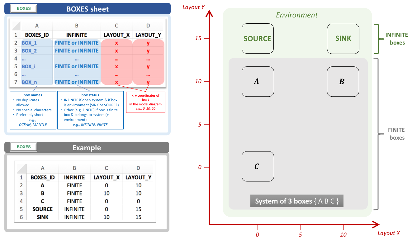
FORCING_SIZE <-
  data.frame(BOXES_ID = c("BOX_1", "...", "BOX_i", "..."),
             SIZE_INIT = c("updated_size_1", "...", "updated_size_i", "..."))

FORCING_SIZE
#>   BOXES_ID      SIZE_INIT
#> 1    BOX_1 updated_size_1
#> 2      ...            ...
#> 3    BOX_i updated_size_i
#> 4      ...            ...
For the 3-boxes closed system model (ABC), in order to change the size of box C from 2000 mg of Ca (default as specified in isobxr master file for all flux lists of FLUXES sheet) to 3000 mg of Ca, the data frame should be structured as follows:
FORCING_SIZE <-
  data.frame(BOXES_ID = c("C"),
             SIZE_INIT = c(3000))

FORCING_SIZE
#>   BOXES_ID SIZE_INIT
#> 1        C      3000
4.3.2 Forcing initial delta values
By default, the run_isobxr function sets the initial
delta values of all boxes at 0 ‰.
It is possible to manually overwrite the initial delta values of one,
several or all boxes for a given run performed by
run_isobxr.
It is done by defining a data frame structured as follows.
FORCING_DELTA <-
  data.frame(BOXES_ID = c("BOX_1", "...", "BOX_i", "..."),
             DELTA_INIT = c("updated_delta_1", "...", "updated_delta_i", "..."))

FORCING_DELTA
#>   BOXES_ID      DELTA_INIT
#> 1    BOX_1 updated_delta_1
#> 2      ...             ...
#> 3    BOX_i updated_delta_i
#> 4      ...             ...
For the 3-boxes closed system model (ABC), in order to force initial isotope composition of box A to -1‰, and leave B and C initial values at 0‰, the data frame should be structured as follows:
FORCING_DELTA <-
  data.frame(BOXES_ID = c("A"),
             DELTA_INIT = c(-1))

FORCING_DELTA
#>   BOXES_ID DELTA_INIT
#> 1        A         -1
4.3.3 Forcing fractionation coefficients
By default, the run_isobxr function sets the isotope
fractionation coefficients at the values found in the coefficients list
specified by user.
It is possible to manually overwrite the fractionation coefficients
of one, several or all pairs of boxes for a given run performed by
run_isobxr.
It is done by defining a data frame structured as follows.
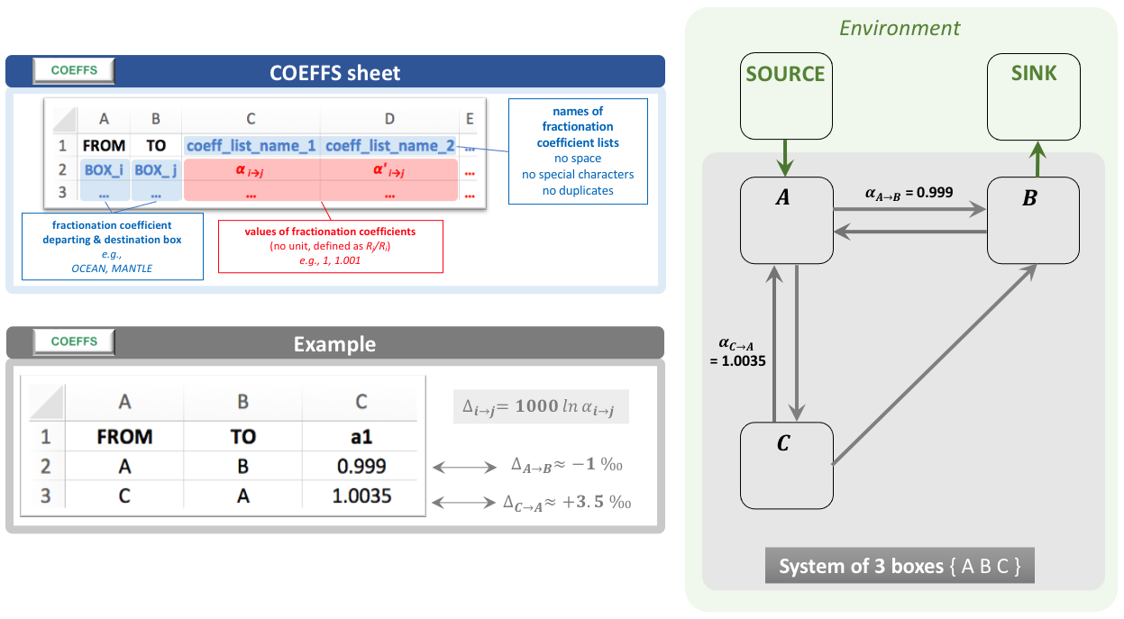
FORCING_ALPHA <-
  data.frame(FROM = c("BOX_i", "..."),
             TO = c("BOX_j", "..."),
             ALPHA = c("new_coeff_value", "..."),
             FROM_TO = c("BOX_i_BOX_j", "..."))

FORCING_ALPHA
#>    FROM    TO           ALPHA     FROM_TO
#> 1 BOX_i BOX_j new_coeff_value BOX_i_BOX_j
#> 2   ...   ...             ...         ...
For the 3-boxes closed system model (ABC), in order to force the fractionation coefficient associated to the flux of Ca from box A to B to the value of 1.02, the data frame should be structured as follows:
FORCING_ALPHA <-
  data.frame(FROM = c("A"),
             TO = c("B"),
             ALPHA = c(1.02),
             FROM_TO = c("A_B"))

FORCING_ALPHA
#>   FROM TO ALPHA FROM_TO
#> 1    A  B  1.02     A_B
4.3.4 Rayleigh distillation models
It is possible to overwrite isotope fractionation coefficients by defining their values as the result of Rayleigh type isotope distillation in the context of a fractional exchange at an interface.
We consider here the case of the loss of element X from a box A to a box C through an interface box B, all possibly part of a bigger box model system.
We suppose that the apparent fractionation coefficient \(\alpha_{A \to C}\) associated to this flux \(F_{A \to C}\) results from a Rayleigh type distillation occurring during the fractional exchange of element X at the interface box B.

In this situation, the box A exchanges element X with box B (and possibly other boxes).
This is a fractional exchange, i.e. during this exchange, box A sends more of element X to box B than B sends back (\(F_{A \to B} > F_{B \to A}\)).
As we consider box B to be balanced, it loses the difference to box C: \(F_{B \to C} = F_{A \to B} - F_{B \to A}\).
As a result, box A loses a total of \(F_{B \to C}\) of element X per time unit.
We suppose here that the \(F_{A \to B}\) that feeds box B is associated to no isotope fractionation.
On the other hand, we suppose that the \(F_{B \to A}\) flux corresponding to the fractional loss of element X from interface box B, and returning to box A, is associated to an equilibrium or incremental isotope fractionation (\(\alpha^0 _{B \to A}\)).
The Rayleigh distillation model of isotopes thus predicts the following:
\[R_{C} = R_{C, t_0} \dfrac{F_{B \to C}}{F_{A \to B}}^{\alpha^0 _{B \to A} - 1} \]
The \(R_{C, t_0}\) corresponds to the isotope ratio of the element X in box B before any exchange with box A occurs. It is thus equivalent to \(R_{A}\) since the box B only input is via the \(F_{A \to B}\) flux.
We thus can write the following definition of \(\alpha_{B \to C}\) (equivalent here to \(\alpha_{A \to C}\)):
\(\alpha_{B \to C} = \dfrac{R_{C}}{R_{A}} = \dfrac{F_{B \to C}}{F_{A \to B}}^{\alpha^0 _{B \to A} - 1}\)
The run_isobxr function here takes as an optional input
the data frame structured as follows:
FORCING_RAYLEIGH <-
  data.frame(XFROM = c("B"), # Define the B>C flux at numerator
             XTO = c("C"),
             YFROM = c("A"), # Define the A>B flux at denominator
             YTO = c("B"),
             AFROM = c("B"), # Define the resulting fractionation coefficient
             ATO = c("C"),
             ALPHA_0 = c("a0") # Define the value of incremental B>A coefficient
  )

FORCING_RAYLEIGH
#>   XFROM XTO YFROM YTO AFROM ATO ALPHA_0
#> 1     B   C     A   B     B   C      a0
The run_isobxr function will in this case overwrite the
value of \(\alpha_{B \to C}\) set in
isobxr master file or using the FORCING_ALPHA
parameter.
Indeed, if the user forced a new value for \(\alpha_{B \to C}\) using the FORCING_ALPHA
parameter, the run_isobxr function will prioritize the
FORCING_RAYLEIGH parameter.
It is possible to define several Rayleigh distillation apparent
fractionation coefficients in a given model.
This is done by adding rows to this data frame.