6 - compose_isobxr: tutorial
Théo Tacail
This vignette is designed to drive the user through a step-by-step
tutorial for the use of the compose_isobxr function.
The user can run the same box model simulations as described in this vignette using the tutorial mode or using the tutorial files.
The user can also find general information about the
compose_isobxr function in the 5
- compose_isobxr: presentation documentation.
1 Prepare tutorial
If not done yet, install the isobxr package (installation instructions here).
Load isobxr in R:
library(isobxr)- If you use the tutorial mode, the tutorial files are called by setting the workdir argument as follows:
workdir <- "/Users/username/Documents/1_ABC_tutorial"
# or
workdir <- "use_isobxr_demonstration_files"
If done so, the following steps can be skipped.
Alternatively, download the tutorial files.
Unzip the ABC tutorial file and place it in the working directory of your choice.
- Note
- It is strongly advised to avoid use a working directory actively linked to an online backup server (such as OneDrive). This could cause some conflict issues with adressing of output files. If done so, users are advised to turn the backup server software offline during the use of isobxr.
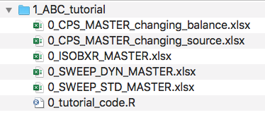
- Go through folder contents:
- Excel master files for the tutorials of each function.
- Including 0_ISOBXR_MASTER.xlsx which defines the systems modelled in this tutorial.
- A R code file (0_tutorial_code.R) which regroups all R commands called throughout all tutorials.
Open the R code file (0_tutorial_code.R) with Rstudio.
Update the correct working directory path to the 1_ABC_tutorial folder
This could for instance look like:
workdir <- "/Users/username/Documents/1_ABC_tutorial"2 System definition
The system we consider in this tutorial is the same as the one defined in the example #3 of run_isobxr tutorial.
We consider a system composed of 3 finite boxes (A, B and C), exchanging with the environment (SOURCE and SINK boxes).
The fluxes of Ca between the finite boxes are balanced and defined by the “Fx3_ABC_open_bal” flux_list by default.
We consider by default the “a1” coeff_list which determines an isotope fractionation of -1‰ associated with the flux from box C to box A.
These system definitions are stored in the 0_ISOBXR_MASTER.xlsx file.
3 Ex. 1: Changing intensity of fluxes
In this tutorial, we will use :
- the 0_ISOBXR_MASTER.xlsx file found in the 1_ABC_tutorial folder
- the 0_CPS_MASTER_changing_balance.xlsx compose master file found in the 1_ABC_tutorial folder
3.1 Define the scenario
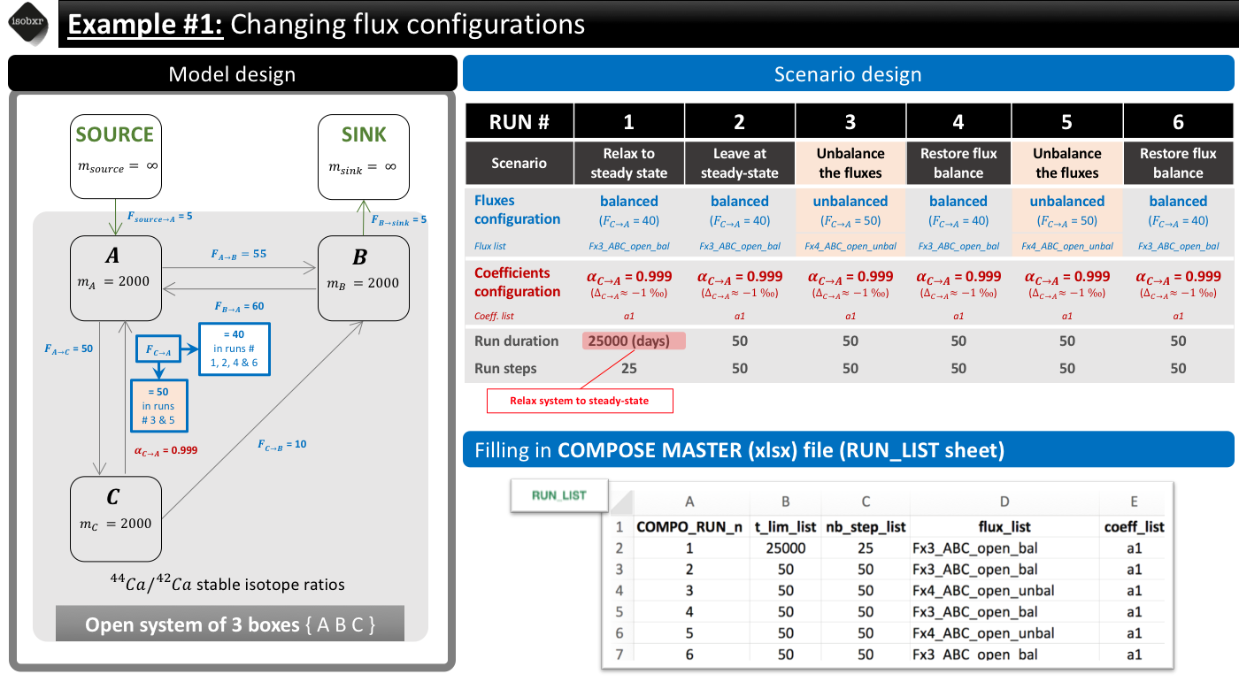
In this first scenario, we want to change the intensity of one flux (from box C to A), therefore provoking an imbalance in the configurations of fluxes between finite boxes.
To do so, we build the following scenario.
Run 1: We want to let the system relax to its steady state. We therefore let the balanced fluxes (flux_list “Fx3_ABC_open_bal”) and the desired fractionation coefficient (coeff_list : “a1”). We define a long run duration (25000 days, 25 steps) in order to reach steady-state. This initial run is used as a primer in order to reach equilibrium but this relaxation will not be considered in the default graphical outputs.
Run 2: We let the system evolve at steady-state in the exact same conditions in order to include a baseline in the default graphical outputs. We let it run for 50 days (50 steps).
Run 3: We change the value of the flux from C to A to 50 mg/d (flux_list: “Fx4_ABC_open_unbal”), initially set at 40 mg/d (in flux_list: “Fx3_ABC_open_bal”). We let this run during 50 days (50 steps).
Run 4: We change the value of the flux back to the balanced configuration initially set at 40 mg/d (in flux_list: “Fx3_ABC_open_bal”). We let this run during 50 days (50 steps).
Run 5: We change the value of the flux from C to A to 50 mg/d (flux_list: “Fx4_ABC_open_unbal”), initially set at 40 mg/d (in flux_list: “Fx3_ABC_open_bal”). We let this run during 50 days (50 steps).
Run 6: We change the value of the flux back to the balanced configuration initially set at 40 mg/d (in flux_list: “Fx3_ABC_open_bal”). We let this run during 50 days (50 steps).
The overview of the scenario is given below together with the corresponding filling of the compose master file.
The following animation pinpoints the different definitions of the system at the 6 stages of the scenario.
3.2 Filling in the compose master file
As we only change the flux configurations in this scenario, we only need to fill in the RUN_LIST sheet. We don’t need the optional forcings also possible with compose_isobxr. The corresponding forcing spreadsheets (FORCING_SIZE, FORCING_DELTA, FORCING_ALPHA, FORCING_RAYLEIGH) are thus left empty with headers only in the compose master file. You can see that in the compose master file of this file.
The RUN_LIST can thus be filled as shown in the scenario overview.
The compose master file for this tutorial is the 0_CPS_MASTER_changing_balance.xlsx file. You can open it, read and play with it.
3.3 Calling compose_isobxr
We can run the model by defining the various required (and optional)
parameters for the compose_isobxr function.
This code can be found in the 0_tutorial_code.R also found in the 1_ABC_tutorial folder.
compose_isobxr(workdir = "/Users/username/Documents/1_ABC_tutorial", # directory containing master files
               SERIES_ID = "ABC_change_balance", # name of the series ID
               time_units = c("d", "d"), # in/out time units for pdf plots
               COMPO_MASTER = "0_CPS_MASTER_changing_balance.xlsx",
               plot_HIDE_BOXES_delta = c("SINK"), # hide in delta plots
               plot_HIDE_BOXES_size = c("SOURCE", "SINK"), # hide in size plots
               EACH_RUN_DIGEST = FALSE, # export the DIGEST for each run
to_CPS_DIGEST_CSVs = TRUE) # export whole model to CSVs- R console messages
-
The first default outputs are messages printed on the R console. The
messages returned by
compose_isobxrare the following:
06_cps_ex1_message
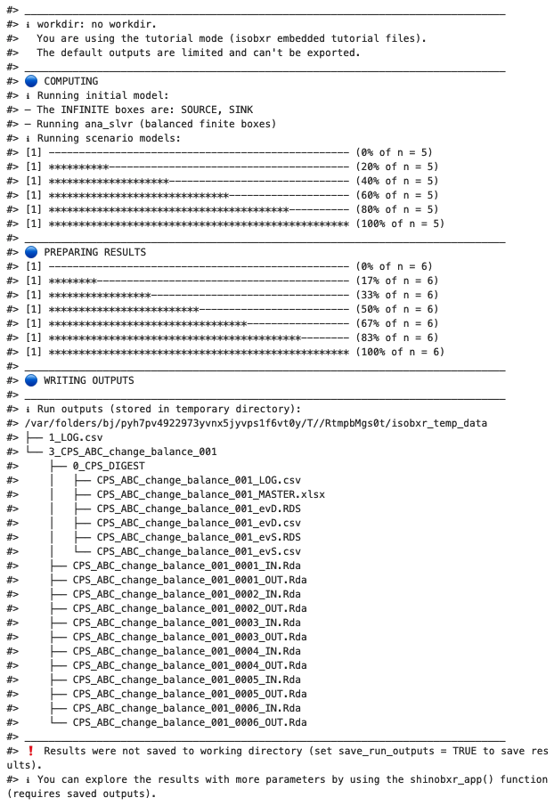
The function reminds us the working directory currently in use (in this case it is the tutorial mode)
The function informs us of the different steps of calculation (computing, preparation of results, output writing to temporary directory)
The function displays the list of the output files produced by the run.
The function informs us about the status of the output file saving, here the files were not saved to any local working directory (as the save_run_outputs = FALSE by default and this is a tutorial mode)
3.4 Run outputs
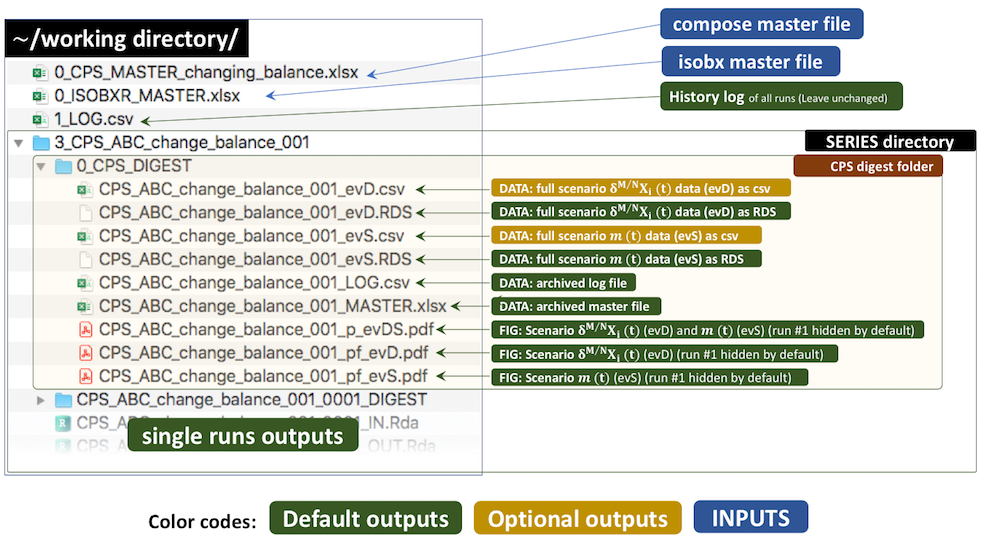
The outputs of this run are kept by default in a temporary directory. Outside tutorial mode (if workdir is referring to a local directory), the user can save these outputs to the working directory by setting the save_run_outputs argument to TRUE. These outputs are structured as follows:
3.5 Plots
You can find the default plot named “…_p_evDS.pdf” which gives the overview of the evolution of delta values and masses of element X in all (non hidden) boxes through time. For this scenario, this should look like this.
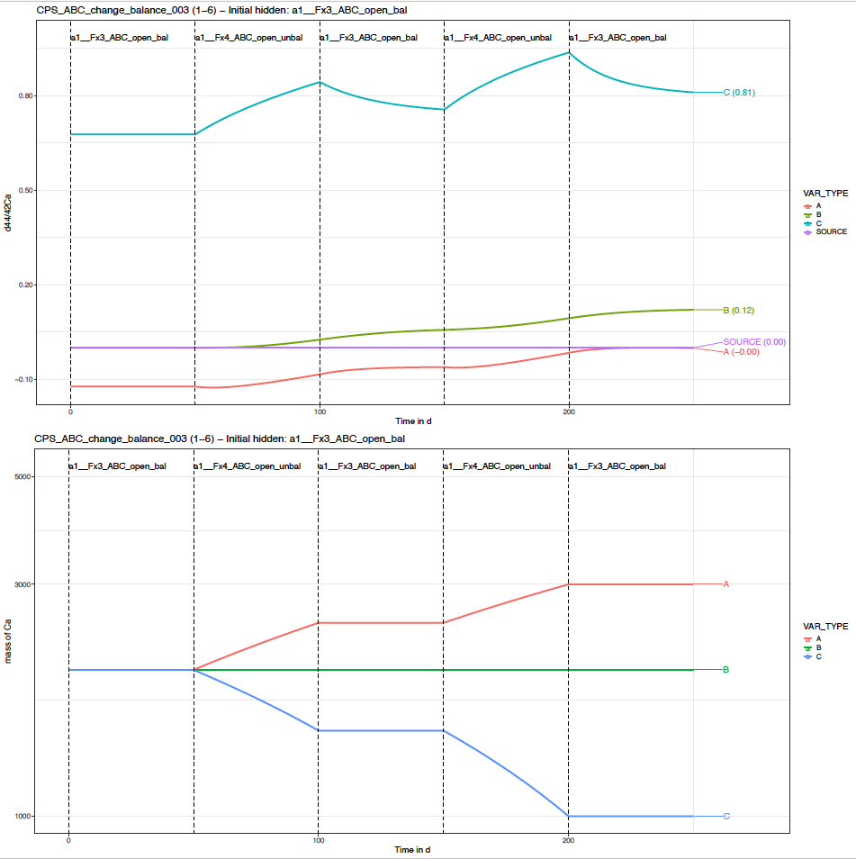
In the top graph, we see that the delta values are markedly affected by the change in the intensity of the flux of Ca from box C to A, especially in box C, but this propagates also to boxes A and B.
In the bottom graph, we see that the sizes of boxes C and A changed. This is expected. The box A is gaining Ca as the unbalanced configuration induces a positive balance of box A. The box C is losing Ca as the unbalanced configuration induces a negative balance of box C.
3.6 Run plotting shiny app
You can run the shinobxr_app function in order to edit
the compose_isobxr output plots and export them as pdf.
This app uses any internet browser but will work offline, and therefore
does not imply the uploading of data.
To do so, you need to store working directory in the workdir variable. This corresponds to the workdir defined where output files were saved (if save_run_outputs = TRUE), for instance:
workdir <- "/Users/username/Documents/any_directory_of_your_choice/1_ABC_tutorial"You can then call the shinobxr_app function which will
open a window in your default internet browser and follow the
instructions shown in the app.
shinobxr_app()Below is a short introduction to the use of the shiny app for
plotting compose_isobxr outputs, made uisng the current
example.
4 Ex. 2 : Changing source composition
In this tutorial, we will use :
- the 0_ISOBXR_MASTER.xlsx file found in the 1_ABC_tutorial folder
- the 0_CPS_MASTER_changing_source.xlsx compose master file found in the 1_ABC_tutorial folder
4.1 Define the scenario
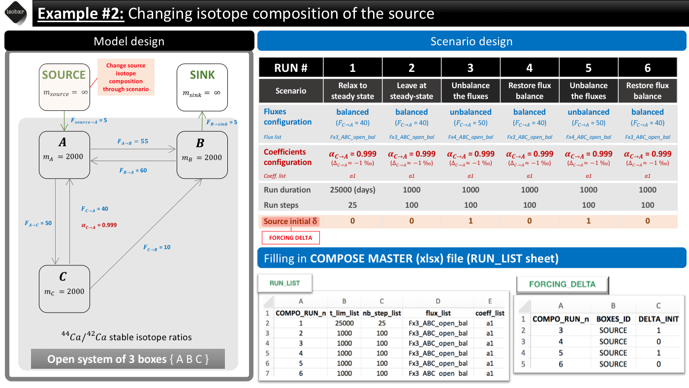
In this first scenario, we want to change the isotope composition of the source (SOURCE box) and see how the whole system reacts to these changes. We aim at inducing a step function changing the source isotope composition from 0 to 1‰ twice.
To do so, we build the following scenario.
Run 1: We want to let the system relax to its steady state. We therefore let the balanced fluxes (flux_list “Fx3_ABC_open_bal”) and the desired fractionation coefficient (coeff_list : “a1”). We define a long run duration (25000 days, 25 steps) in order to reach steady-state. This initial run is used as a primer in order to reach equilibrium but this relaxation will not be considered in the default graphical outputs.
Run 2: We let the system evolve at steady-state in the exact same conditions in order to include a baseline in the default graphical outputs. We let it run for 1000 days (100 steps).
Run 3: We force the run initial isotope composition of the SOURCE box to 1‰ (instead of 0‰ as was by default previously). We let it run for 1000 days (100 steps).
Run 4: We force the run initial isotope composition of the SOURCE box back to 0‰. We let it run for 1000 days (100 steps).
Run 5: We force the run initial isotope composition of the SOURCE box again to 1‰. We let it run for 1000 days (100 steps).
Run 6: We force the run initial isotope composition of the SOURCE box back to 0‰. We let it run for 1000 days (100 steps).
The overview of the scenario is given below together with the corresponding filling of the compose master file.
The following animation pinpoints the different definitions of the system at the 6 stages of the scenario.
4.2 Filling in the compose master file
As the scenario is defined by the system global definitions but also with an additional forcing of the runs initial delta values, you need to both fill in the RUN_LIST sheet and the FORCING_DELTA sheet.
The RUN_LIST can thus be filled as shown in the scenario overview.
The FORCING_DELTA can thus be filled as shown in the scenario overview.
The compose master file for this tutorial is the 0_CPS_MASTER_changing_source.xlsx file. You can open it, read and play with it.
4.3 Calling compose_isobxr
We can run the model by defining the various required (and optional)
parameters for the compose_isobxr function.
This code can be found in the 0_tutorial_code.R also found in the 1_ABC_tutorial folder.
compose_isobxr(workdir = "/Users/username/Documents/1_ABC_tutorial",
               SERIES_ID = "ABC_change_source", # name of the series ID
               time_units = c("d", "yr"), # in/out time units for pdf plots
               COMPO_MASTER = "0_CPS_MASTER_changing_source.xlsx", # compose master file
               plot_HIDE_BOXES_delta = c("SINK"), # hide in delta plots
               plot_HIDE_BOXES_size = c("SOURCE", "SINK"), # hide in size plots
               EACH_RUN_DIGEST = FALSE, # export the DIGEST for each run
to_CPS_DIGEST_CSVs = TRUE) # export whole model to CSVs- R console messages
-
The first default outputs are messages printed on the R console. The
messages returned by
compose_isobxrare the following:
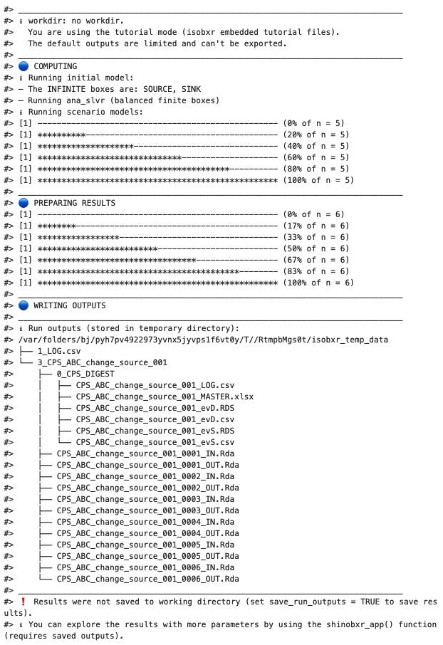
The function reminds us the working directory currently in use (in this case it is the tutorial mode)
The function informs us of the different steps of calculation (computing, preparation of results, output writing to temporary directory)
The function displays the list of the output files produced by the run.
The function informs us about the status of the output file saving, here the files were not saved to any local working directory (as the save_run_outputs = FALSE by default and this is a tutorial mode)
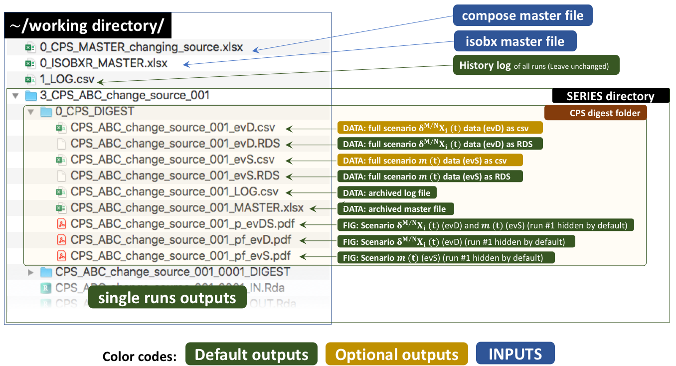
4.4 Run outputs
The outputs of this run are kept by default in a temporary directory. Outside tutorial mode (if workdir is referring to a local directory), the user can save these outputs to the working directory by setting the save_run_outputs argument to TRUE. These outputs are structured as follows:
4.5 Plots
You can find the default plot named “…_p_evDS.pdf” which gives the overview of the evolution of delta values and masses of element X in all (non hidden) boxes through time. For this scenario, this should look like this.
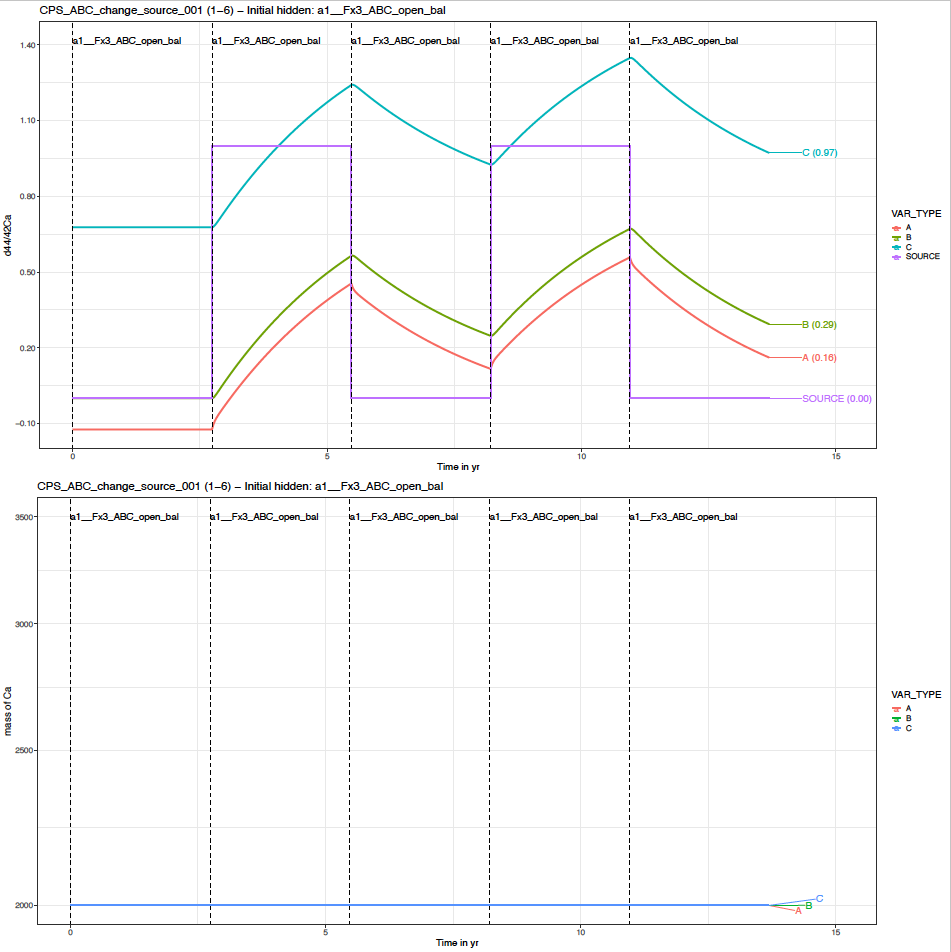
In the top graph, we see that the delta values are markedly affected by the step changes in the SOURCE delta values.
In the bottom graph, we see that the sizes of boxes remain unchanged. This is expected since the system remained in a balanced flux configuration.
4.6 Run plotting shiny app
You can run the shinobxr_app function in order to edit
the compose_isobxr output plots and export them as pdf.
This app uses any internet browser but will work offline, and therefore
does not imply the uploading of data.
To do so, you need to store working directory in the workdir variable. This corresponds to the workdir defined where output files were saved (if save_run_outputs = TRUE), for instance:
workdir <- "/Users/username/Documents/any_directory_of_your_choice/1_ABC_tutorial"You can then call the shinobxr_app function which will
open a window in your default internet browser and follow the
instructions shown in the app.
shinobxr_app()Below is a short introduction to the use of the shiny app for
plotting compose_isobxr outputs, made uisng the current
example.