This vignette is designed to drive the user through a step-by-step tutorial for the use of the run_isobxr function.

The user can run the same box model simulations as described in this vignette using the tutorial mode or using the tutorial files.

The user can also find general information about the run_isobxr function in the 3 - Run_isobxr: presentation vignette.

1 Prepare tutorial

If not done yet, install the isobxr package (installation instructions here).
Load isobxr in R:

library(isobxr)

If you use the tutorial mode, the tutorial files are called by setting the workdir argument as follows:

workdir <- "/Users/username/Documents/1_ABC_tutorial"
# or
workdir <- "use_isobxr_demonstration_files"

If done so, the following steps can be skipped.

Alternatively, download the tutorial files.
Unzip the ABC tutorial file and place it in the working directory of your choice.

Note: It is strongly advised to avoid use a working directory actively linked to an online backup server (such as OneDrive). This could cause some conflict issues with adressing of output files. If done so, users are advised to turn the backup server software offline during the use of isobxr.

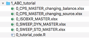
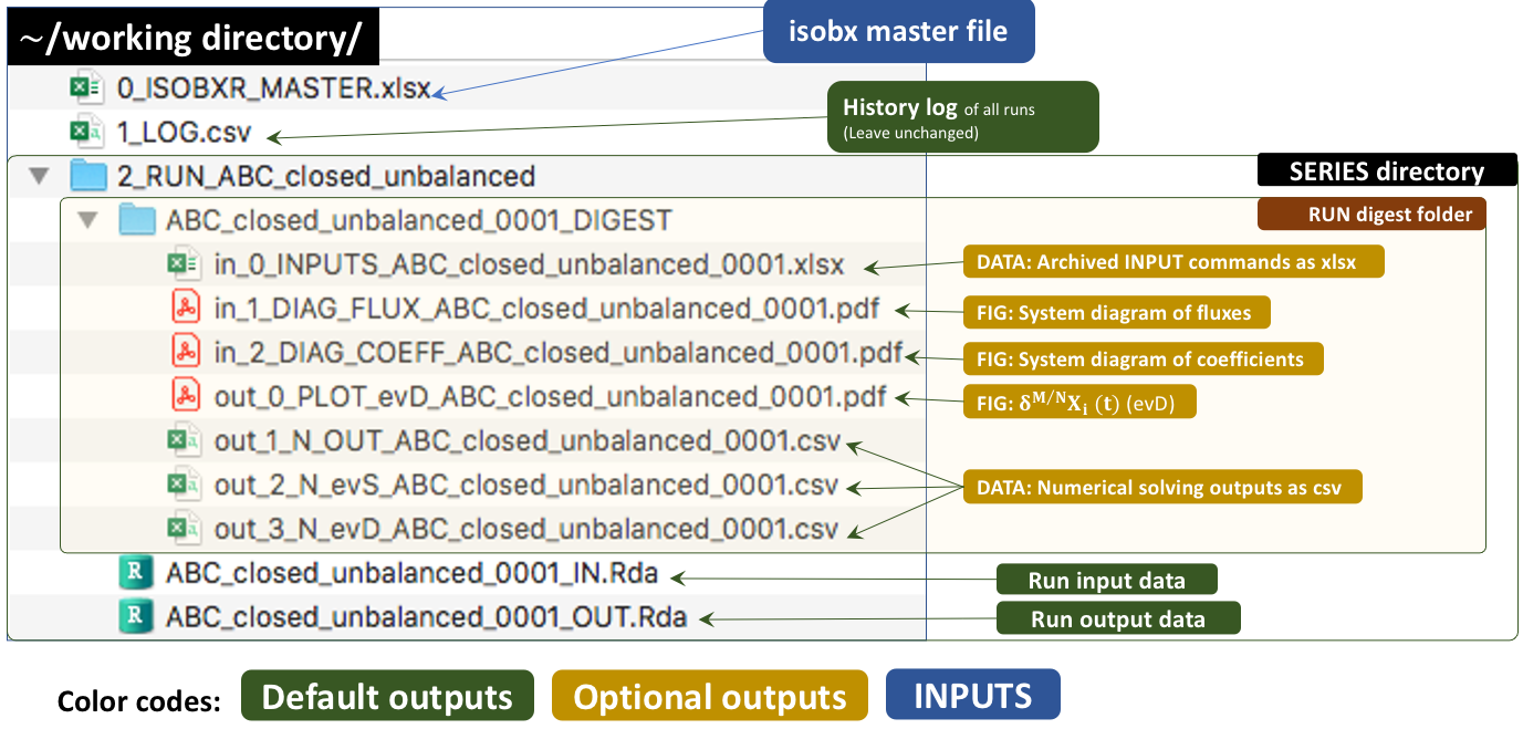
Go through folder contents:

Excel master files for the tutorials of each function.
Including 0_ISOBXR_MASTER.xlsx which defines the systems modelled in this tutorial.
A R code file (0_tutorial_code.R) which regroups all R commands called throughout all tutorials.

Open the R code file (0_tutorial_code.R) with Rstudio.
Update the correct working directory path to the 1_ABC_tutorial folder

This could for instance look like:

workdir <- "/Users/username/Documents/1_ABC_tutorial"

2 Ex. 1: {ABC}, closed, balanced

2.1 System definition

We consider here the case a balanced and closed system of 3 finite boxes A, B and C. This system is defined in the 0_ISOBXR_MASTER.xlsx file as follows:

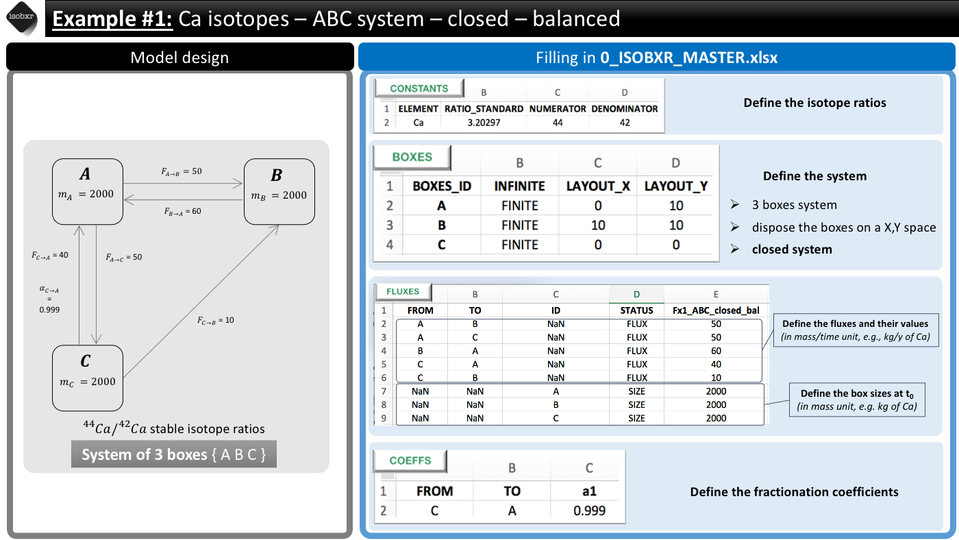
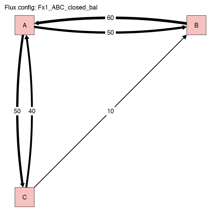
We consider the list of balanced fluxes Fx1_ABC_closed_bal

No box loses nor gains Ca, the system is balanced

For this run we use the a1 fractionation coefficients list

We only define a -1‰ fractionation during transport from box C to A (\(\alpha_{C \to A} = 0.999\))

Units

We consider a system where the fluxes are expressed in mg/d
The masses of Ca in each box (box sizes) are expressed in mg
The run will thus be performed with d as time units

2.2 Run the model

Run duration and resolution

We run this model for total duration of 2500 days
With a resolution of 1 calculation every 10 days, corresponding to 250 steps

Initial state

We don’t force any initial isotope compositions to the system: the initial delta values will be 0‰ by default in all boxes.

Run SERIES ID

We can define the name of the SERIES of run this run will belong to.
We chose a short description (with no special characters): “ABC_closed_balanced”

We can run the model as follows

run_isobxr(workdir = "/Users/username/Documents/1_ABC_tutorial", # work. directory
           SERIES_ID = "ABC_closed_balanced", # name of the series of runs
           flux_list_name = "Fx1_ABC_closed_bal", # use this list of fluxes/sizes
           coeff_list_name = "a1", # use list a1 of fractionation coeffs.
           t_lim = 2500, # run the model over 2500 days
           nb_steps = 250, # calculate system state in 250 steps
           time_units = c("d", "yr"), # run time units (days), plot time units (years)
           to_DIGEST_evD_PLOT = TRUE, # export plot as pdf
           to_DIGEST_CSV_XLS = TRUE, # export all data as csv and xlsx
           to_DIGEST_DIAGRAMS = TRUE) # export system diagrams as pdf

R console messages: The first default outputs are messages printed on the R console. The messages returned by run_isobxr are the following:

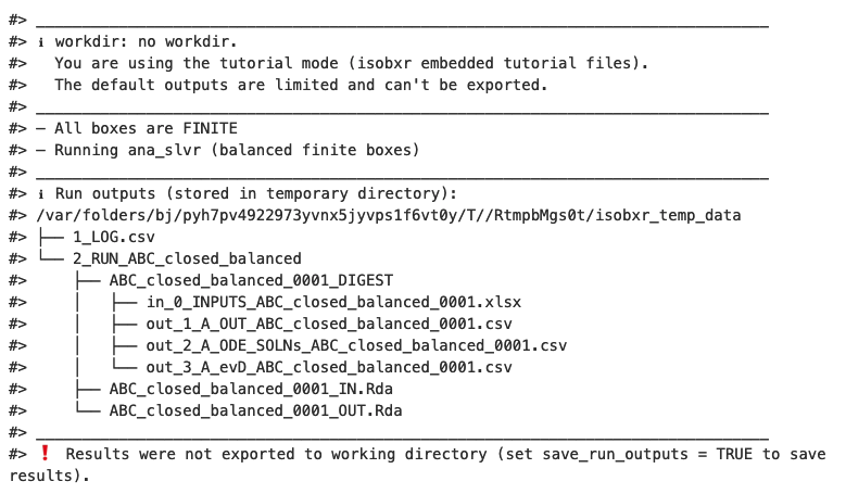
The function reminds us the working directory currently in use (in this case it is the tutorial mode)
The function reports the results of the analysis of the system:
- The {ABC} system being closed, the run_isobxr function identified that all boxes are finite.
- The {ABC} system being balanced, the run_isobxr function identified that the analytical solving of the model can be performed (using the analytical solver ana_slvr).
The function reports the list of output data files produced (stored in a temporary directory, not saved by default).
The function informs us the output data files were not saved.

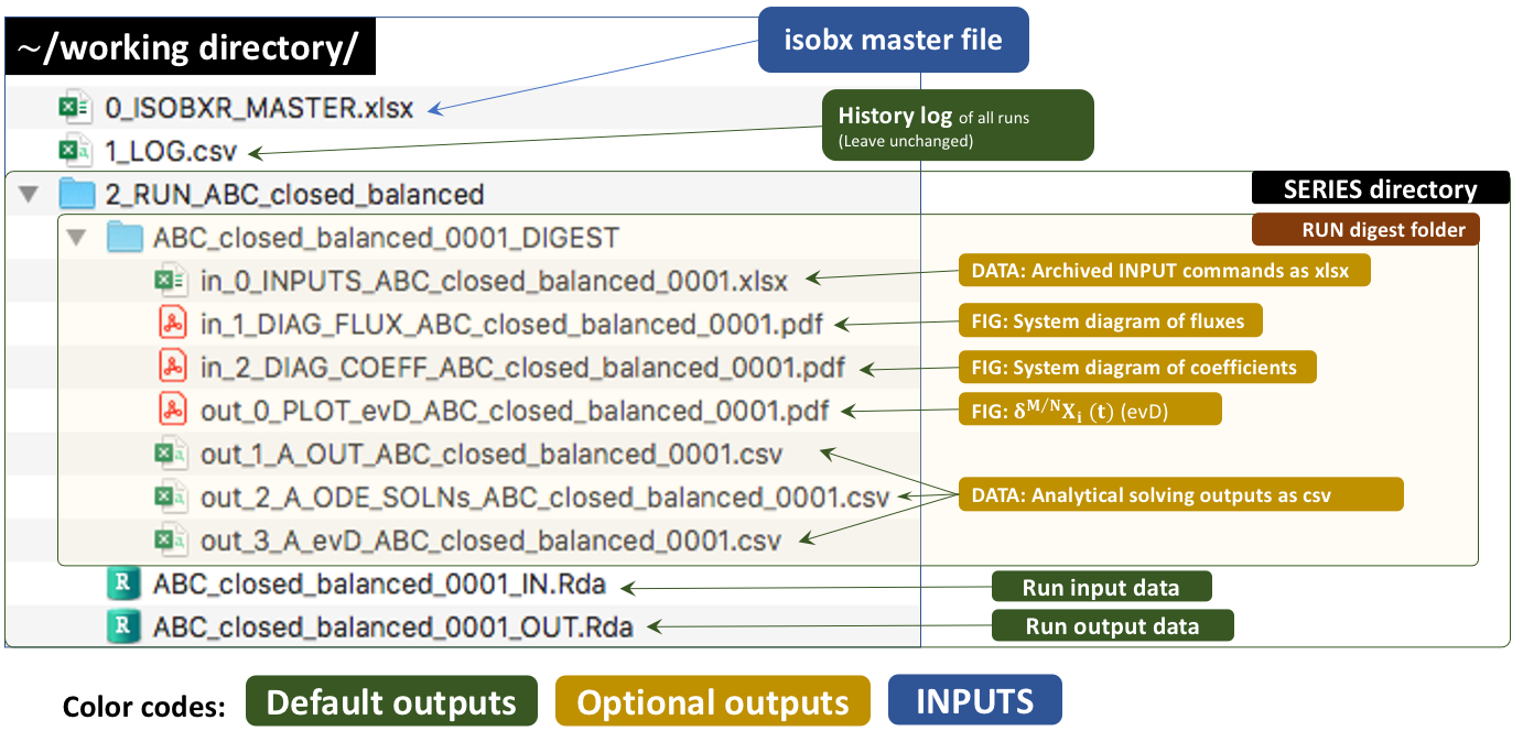
2.3 Run outputs

The outputs of this run are kept by default in a temporary directory. Outside tutorial mode (if workdir is referring to a local directory), the user can save these outputs to the working directory by setting the save_run_outputs argument to TRUE. These outputs are structured as follows:

2.3.1 System diagrams

The run_isobxr function produced an overview of the system as diagrams (pdf) for fluxes (left) and isotope fractionation expressed ‰ (right) shown below:

2.3.2 Plots

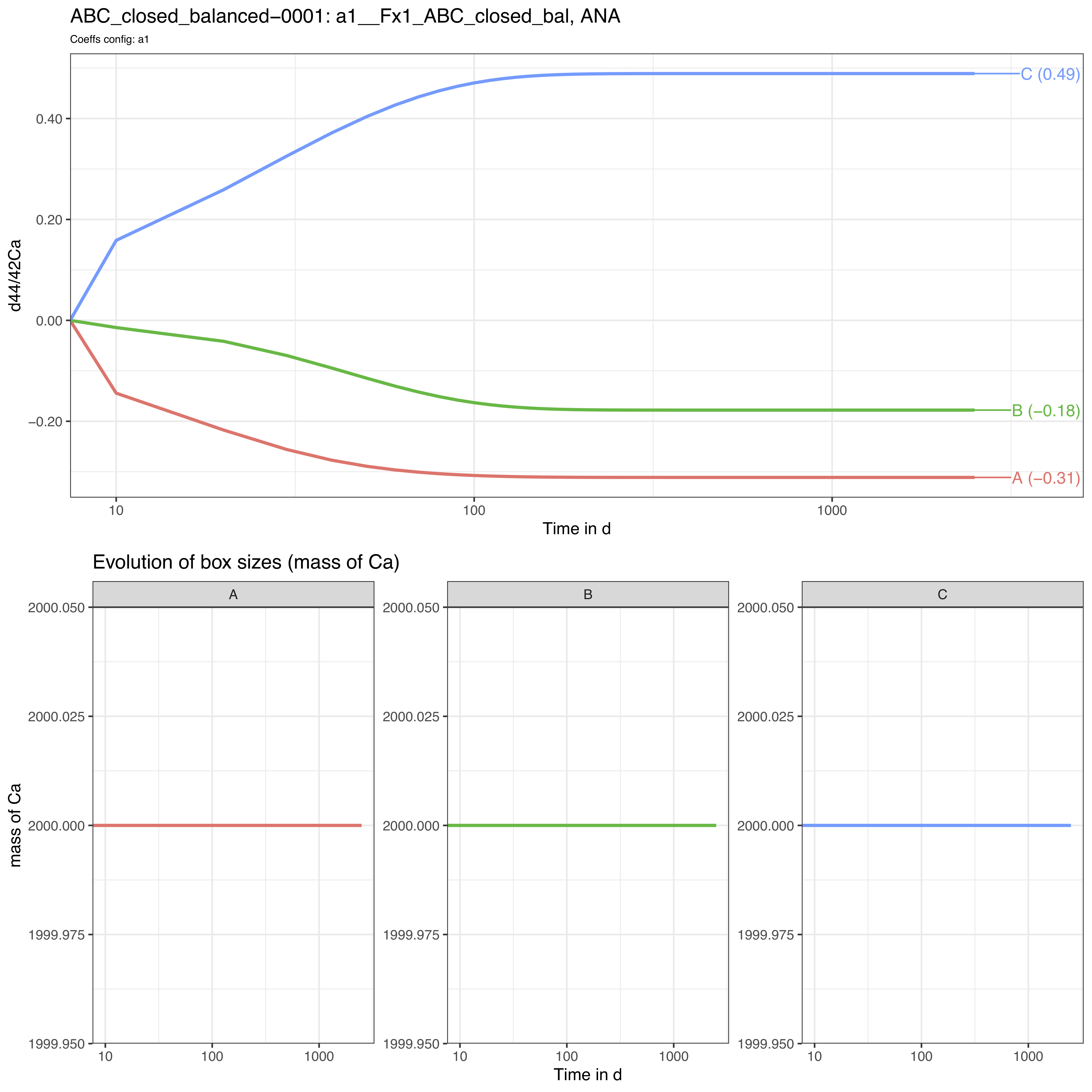
The run_isobxr outputs include the evolution of isotope compositions over the run duration (printed in R session by default, and edited as pdf) together with the evolution of the box sizes (masses of element X).

Note that the time axis is displayed with a log scale by default but this can be changed to a linear time scale by setting the run_isobxr parameter evD_PLOT_time_as_log to FALSE.

We thus observe here a relaxation of the system to a steady-state where box A tends to -0.31‰, B to -0.18‰ and C to 0.49‰.

2.3.3 Optional data outputs

As run_isobxr was run with export of csv and xlsx datasets (to_DIGEST_CSV_XLS = TRUE), this run provides user with the following datasets.

in_0_INPUTS_ABC_closed_balanced_0001.xlsx: An archive of all the commands and system definitions used for the run.
out_1_A_OUT_ABC_closed_balanced_0001.csv: A csv summary initial and final state of the system (box sizes, delta values).
out_2_A_ODE_SOLNs_ABC_closed_balanced_0001.csv: The solutions of the differential equations matrix inversion (analytical solving). This includes eigen-values, -vectors, relaxation times.
out_3_A_evD_ABC_closed_balanced_0001.csv: The dataset of stable isotope compositions (delta values in ‰) in all boxes over run duration.

3 Ex. 2: {ABC}, closed, unbalanced

3.1 System definition

We consider here the case a closed system of 3 finite boxes A, B and C.

The fluxes are however unbalanced: boxes A and C have unbalanced inward and outward fluxes.

This system is defined in the 0_IOSOBXR_MASTER.xlsx file as follows:

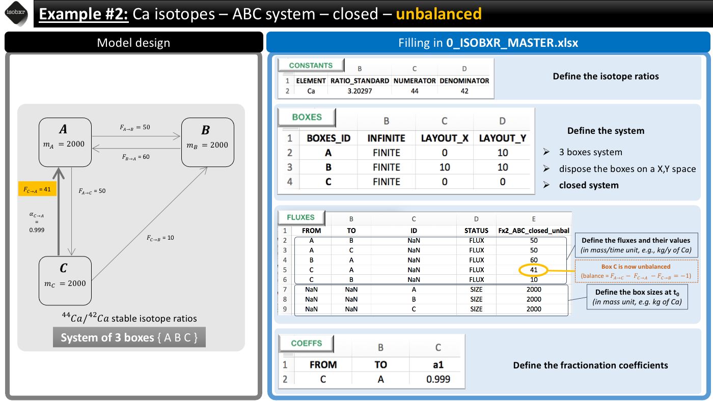
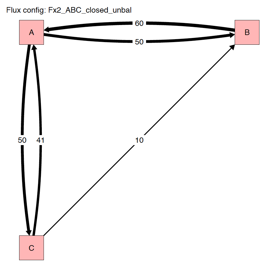
We consider the list of unbalanced fluxes Fx2_ABC_closed_unbal

Box C has a negative balance: it loses 1 mg/d of Ca
Box A has a positive balance: it gains 1 mg/d of Ca

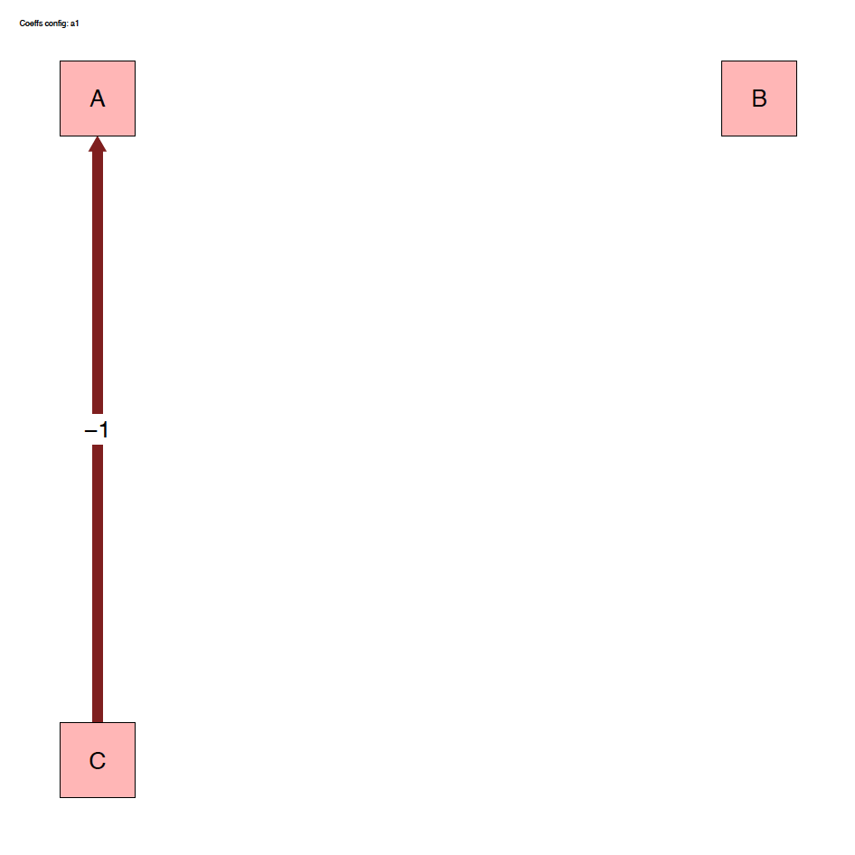
For this run we keep the a1 fractionation coefficients list

We only define a -1‰ fractionation during transport from box C to A (\(\alpha_{C \to A} = 0.999\))

3.2 Run the model

Run duration and resolution

We run this model for total duration of 2500 days
With a resolution of 1 calculation every 10 days, corresponding to 250 steps

Initial state

We don’t force any initial isotope compositions to the system: the initial delta values will be 0‰ by default in all boxes.

Run SERIES ID

We can define the name of the SERIES of run this run will belong to.
We chose a short description (with no special characters): “ABC_closed_unbalanced”

We can run the model as follows

run_isobxr(workdir = "/Users/username/Documents/1_ABC_tutorial", # work. directory
           SERIES_ID = "ABC_closed_unbalanced", # name of the series of runs
           flux_list_name = "Fx2_ABC_closed_unbal", # use this list of fluxes/sizes
           coeff_list_name = "a1", # use list a1 of fractionation coeffs.
           t_lim = 2500, # run the model over 2500 days
           nb_steps = 250, # calculate system state in 250 steps
           time_units = c("d", "yr"), # run time units (days), plot time units (years)
           to_DIGEST_evD_PLOT = TRUE, # export plot as pdf
           to_DIGEST_CSV_XLS = TRUE, # export all data as csv and xlsx
           to_DIGEST_DIAGRAMS = TRUE) # export system diagrams as pdf

R console messages: The first default outputs are messages printed on the R console. The messages returned by run_isobxr are the following:

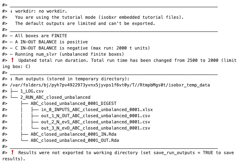
The function reminds us the working directory currently in use (in this case it is the tutorial mode)
The function reports that All boxes are FINITE. This is expected because the {ABC} system being closed, the run_isobxr function identified that all boxes are finite.
However as the system is unbalanced, the run_isobxr function warns the user that:
- Box A has a positive balance
- Box C has a negative balance and would be totally emptied in 2000 days
- Run duration (2500 days) exceeds duration of box C total emptying.
  - As a consequence the function has updated the run duration to the maximum run duration defined by box C emptying.

3.3 Run outputs

3.3.1 System diagrams

The run_isobxr function produced an overview of the system as diagrams (pdf) for fluxes (left) and isotope fractionation expressed ‰ (right) shown below:

3.3.2 Plots

The run_isobxr outputs include the evolution of isotope compositions over the run duration (edited as pdf), shown in years for this run.

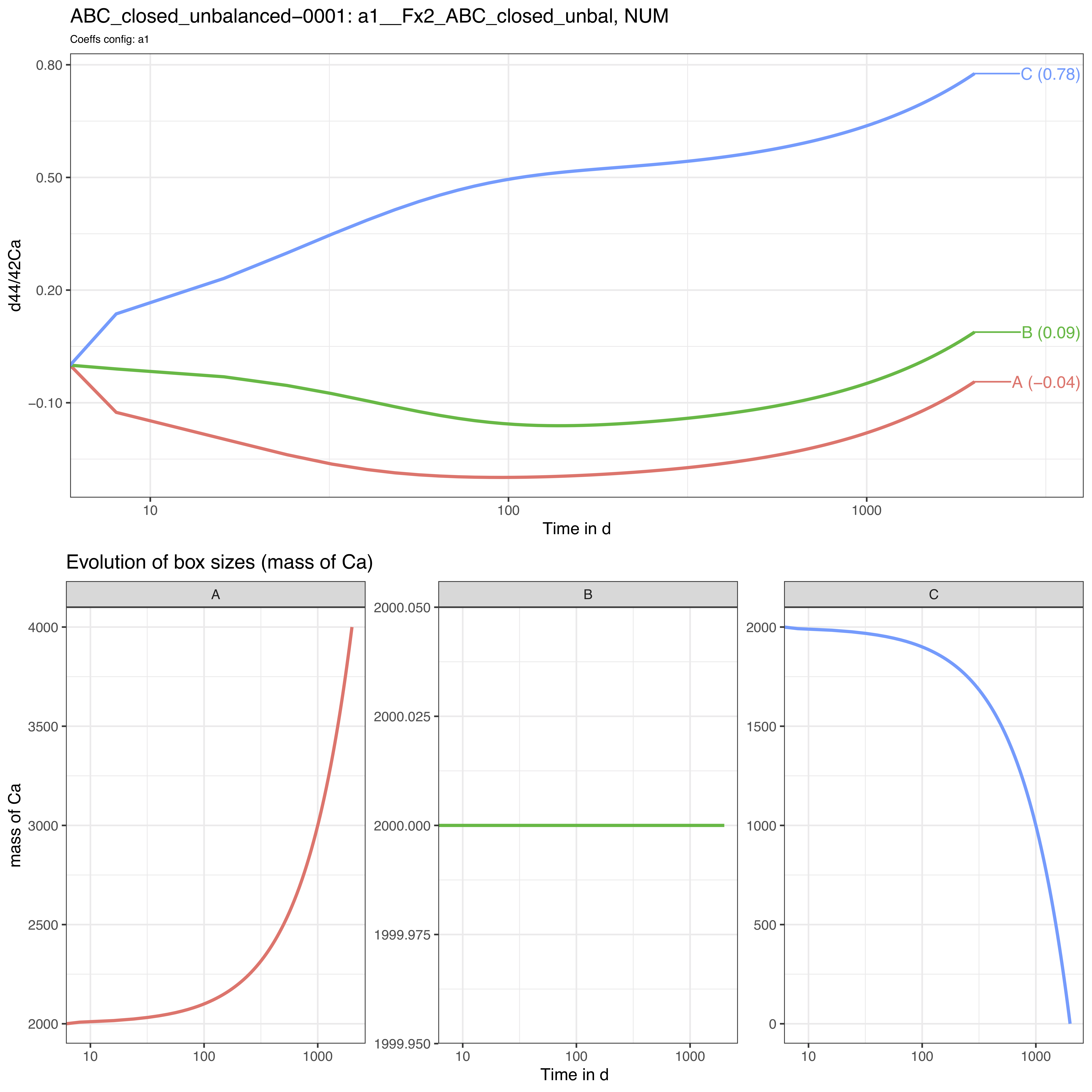
We observe that the box sizes are not constant over time: the box A gains 2000 mass units while the box C is totally emptied by the end of the run.

In this case, we observe here no relaxation to a steady-state.

Note that the time axis is displayed with a log scale by default but this can be changed to a linear time scale by setting the run_isobxr parameter evD_PLOT_time_as_log to FALSE.

3.3.3 Optional data outputs

As run_isobxr was run with export of csv and xlsx datasets (to_DIGEST_CSV_XLS = TRUE), this run provides user with the following datasets.

in_0_INPUTS_ABC_closed_unbalanced_0001.xlsx: An archive of all the commands and system definitions used for the run.
out_1_N_OUT_ABC_closed_unbalanced_0001.csv: A csv summary initial and final state of the system (box sizes, delta values).
out_2_N_evS_ABC_closed_unbalanced_0001.csv: The dataset of box sizes (masses of Ca in mg) in all boxes over run duration.
out_3_N_evD_ABC_closed_unbalanced_0001.csv: The dataset of stable isotope compositions (delta values in ‰) in all boxes over run duration.

4 Ex. 3: {ABC}, open, balanced

4.1 System definition

We consider here the case a balanced system of 3 finite boxes A, B and C.

This system is however open and exchanges Ca with the environment.

This system is defined in the 0_IOSOBXR_MASTER.xlsx file as follows:

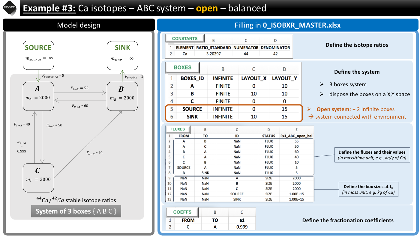
We consider the list of balanced fluxes Fx3_ABC_open_bal: No box loses nor gains Ca, the system is balanced
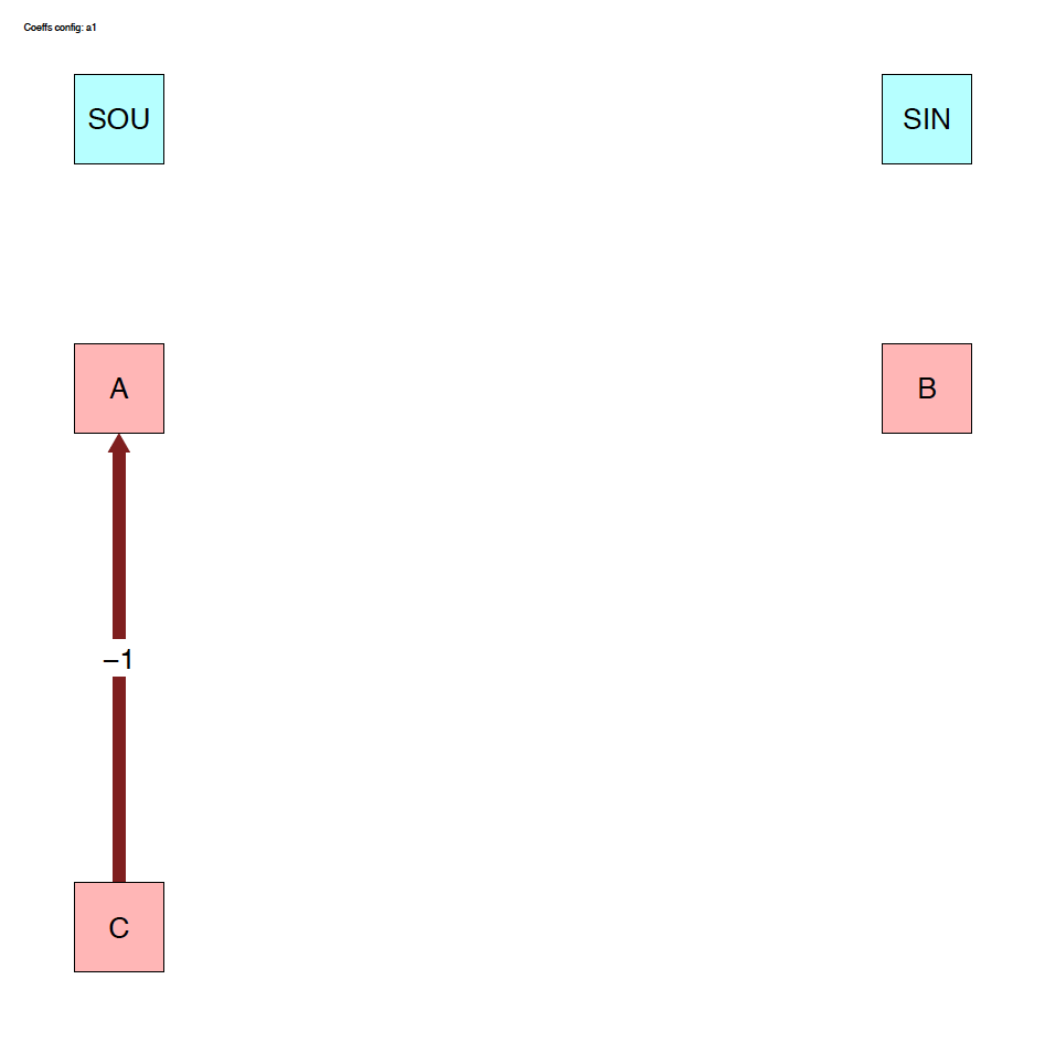
For this run we use the a1 fractionation coefficients list: We only define a -1‰ fractionation during transport from box C to A (\(\alpha_{C \to A} = 0.999\))

4.2 Run the model

Run duration and resolution

We run this model for total duration of 25000 days (longer than previously in examples 1 and 2)
With a resolution of 1 calculation every 10 days, corresponding to 2500 steps

Initial state

We don’t force any initial isotope compositions to the system: the initial delta values will be 0‰ by default in all boxes.

Run SERIES ID

We can define the name of the SERIES of run this run will belong to.
We chose a short description (with no special characters): “ABC_open_balanced”

We can run the model as follows

run_isobxr(workdir = "/Users/username/Documents/1_ABC_tutorial", # work. directory
           SERIES_ID = "ABC_open_balanced", # name of the series of runs
           flux_list_name = "Fx3_ABC_open_bal", # use this list of fluxes/sizes
           coeff_list_name = "a1", # use list a1 of fractionation coeffs.
           t_lim = 25000, # run the model over 2500 days
           nb_steps = 2500, # calculate system state in 250 steps
           time_units = c("d", "yr"), # run time units (days), plot time units (years)
           to_DIGEST_evD_PLOT = TRUE, # export plot as pdf
           to_DIGEST_CSV_XLS = TRUE, # export all data as csv and xlsx
           to_DIGEST_DIAGRAMS = TRUE) # export system diagrams as pdf

R console messages: The first default outputs are messages printed on the R console. The messages returned by run_isobxr are the following:

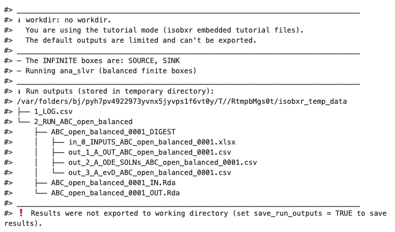
The function reminds us the working directory currently in use (in this case it is the tutorial mode)
The function informs that The INFINITE boxes are: SOURCE, SINK and it is Running ana_slvr (balanced finite boxes). This is expected because:
- The {ABC} system being open, the run_isobxr function identified that SOURCE and SINK are infinite boxes.
- The {ABC} system being balanced, the run_isobxr function identified that the analytical solving of the model can be performed (using the analytical solver ana_slvr).

4.3 Run outputs

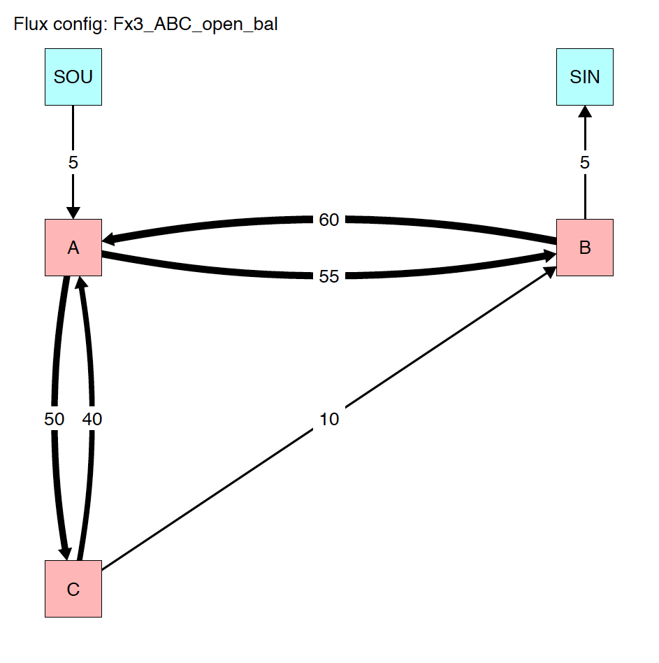
4.3.1 System diagrams

The run_isobxr function produced an overview of the system as diagrams (pdf) for fluxes (left) and isotope fractionation expressed ‰ (right) shown below:

4.3.2 Plots

The run_isobxr outputs include the evolution of isotope compositions over the run duration (edited as pdf), shown in years for this run.

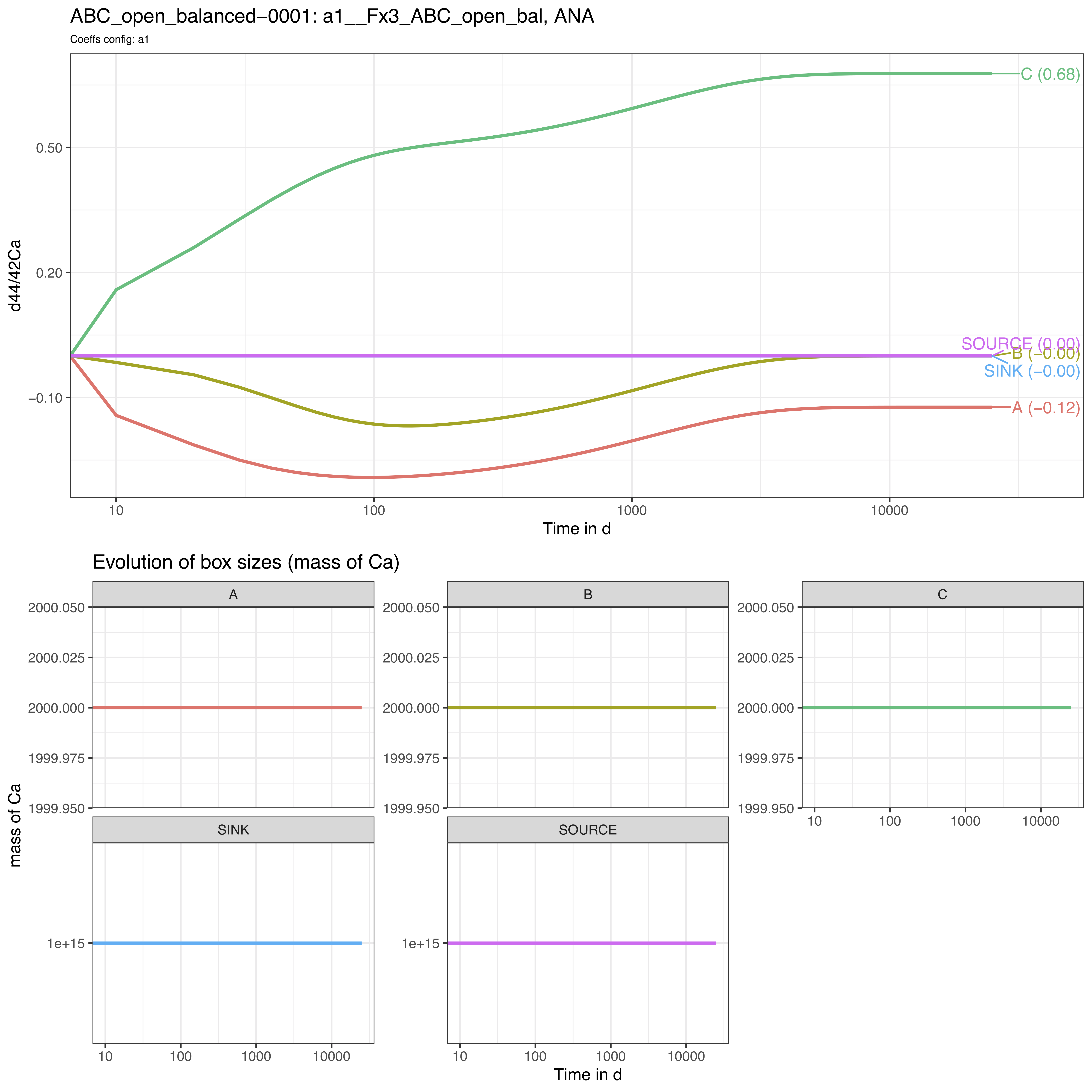
We thus observe here a relaxation of the system to a steady-state (different from example 1) where box A tends to -0.12‰, B to 0‰ and C to +0.68‰.

As we didn’t define the initial isotope compositions of the boxes including the SOURCE and SINK infinite boxes, the later therefore remain at 0‰ throughout the run.

Note that the time axis is displayed with a log scale by default but this can be changed to a linear time scale by setting the run_isobxr parameter evD_PLOT_time_as_log to FALSE.

5 Ex. 4: Add forcing parameters

Additionally to the default definition of the system, it is possible to force other parameters.

Here, we walk you through 2 of the 4 parameters that can be forced with run_isobxr: initial isotope compositions and initial box sizes.

We consider the system of example 3: System {ABC}, open and balanced.

5.1 Forcing deltas

Instead of starting by default with delta values set at 0‰ for all boxes, we want to set:

an initial isotope composition of the SOURCE to -3‰
an initial isotope composition of the box C to +5‰.

To do so we need to define a forcing parameter (FORCING_DELTA) as follows:

FORCING_DELTA <- 
  data.frame(BOXES_ID = c("SOURCE", "C"),
             DELTA_INIT = c(-3, +5))

FORCING_DELTA
#>   BOXES_ID DELTA_INIT
#> 1   SOURCE         -3
#> 2        C          5

We then can run the function and specify the forcing parameter values:

run_isobxr(workdir = "/Users/username/Documents/1_ABC_tutorial", # work. directory
           SERIES_ID = "ABC_open_balanced_w_forcing_delta",
           flux_list_name = "Fx3_ABC_open_bal",
           coeff_list_name = "a1", 
           t_lim = 25000, 
           nb_steps = 2500, 
           time_units = c("d", "yr"), 
           to_DIGEST_evD_PLOT = TRUE, 
           to_DIGEST_CSV_XLS = TRUE,
           to_DIGEST_DIAGRAMS = TRUE, 
           FORCING_DELTA = FORCING_DELTA) # FORCE INITIAL DELTA VALUES

We observe the following evolution of isotope compositions with time:

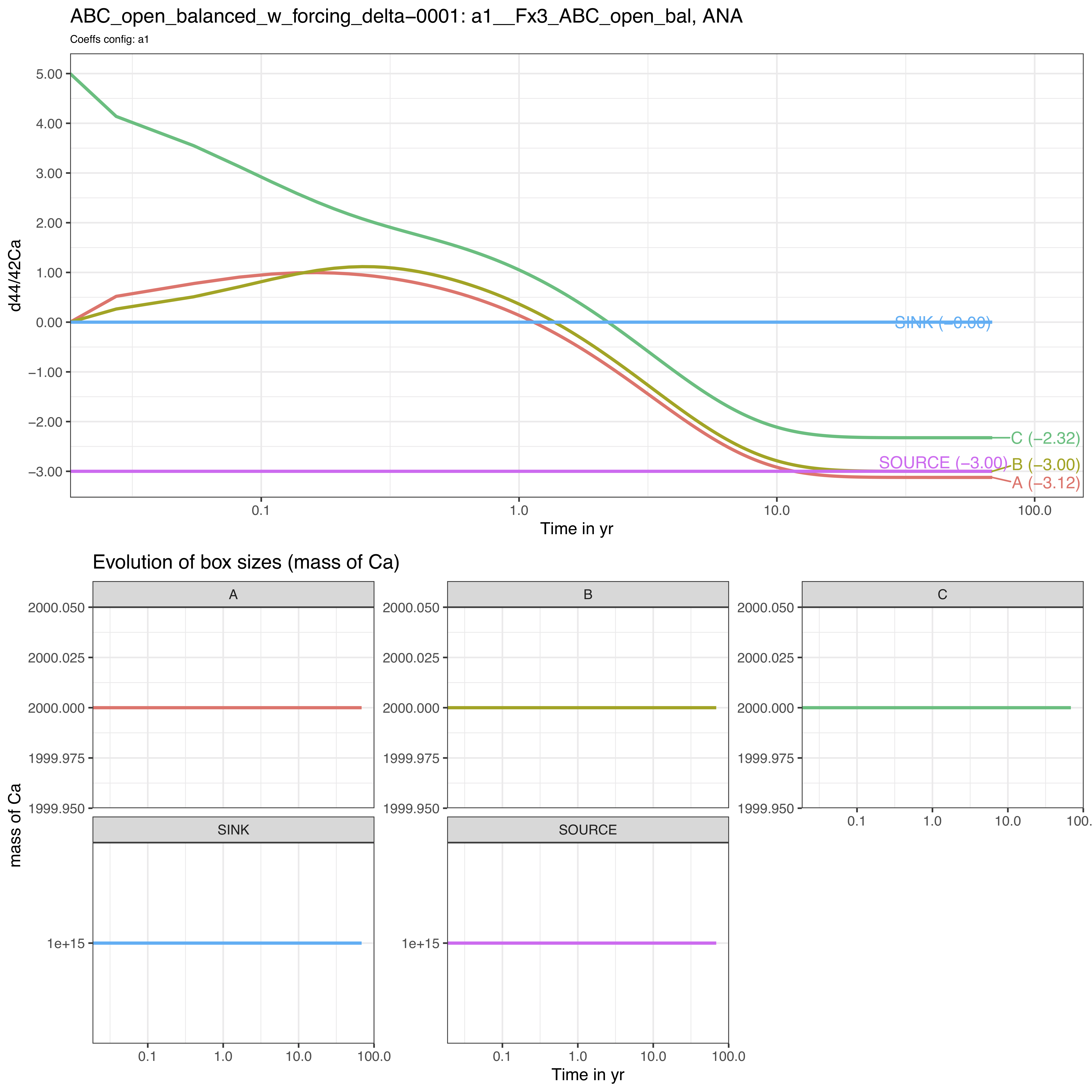
We observe that the box C starts as expected from +5‰ while the steady-state is shifted to lower values by -3‰ since the SOURCE has been set to -3‰.

5.2 Forcing box sizes

Instead of starting by default with box sizes defined in the Fx3_ABC_open_bal flux list of the 0_ISOBXR_MASTER.xlsx file, we modify here the initial sizes of boxes B and C:

B is changed from a size of 2000 to 50
C is changed from a size of 2000 to 1 000 000

To do so we need to define a forcing paramter (FORCING_SIZE) as follows:

FORCING_SIZE <-
  data.frame(BOXES_ID = c("B", "C"),
             SIZE_INIT = c(50, 1e6))

FORCING_SIZE
#>   BOXES_ID SIZE_INIT
#> 1        B     5e+01
#> 2        C     1e+06

We then can run the function and specify the forcing parameter values:

run_isobxr(workdir = "/Users/username/Documents/1_ABC_tutorial", # work. directory
           SERIES_ID = "ABC_open_balanced_w_forcing_size",
           flux_list_name = "Fx3_ABC_open_bal",
           coeff_list_name = "a1", 
           t_lim = 25000, 
           nb_steps = 2500, 
           time_units = c("d", "yr"), 
           to_DIGEST_evD_PLOT = TRUE, 
           to_DIGEST_CSV_XLS = TRUE,
           to_DIGEST_DIAGRAMS = TRUE, 
           FORCING_SIZE = FORCING_SIZE) # FORCE INITIAL SIZE  VALUES

We observe the following evolution of isotope compositions with time:

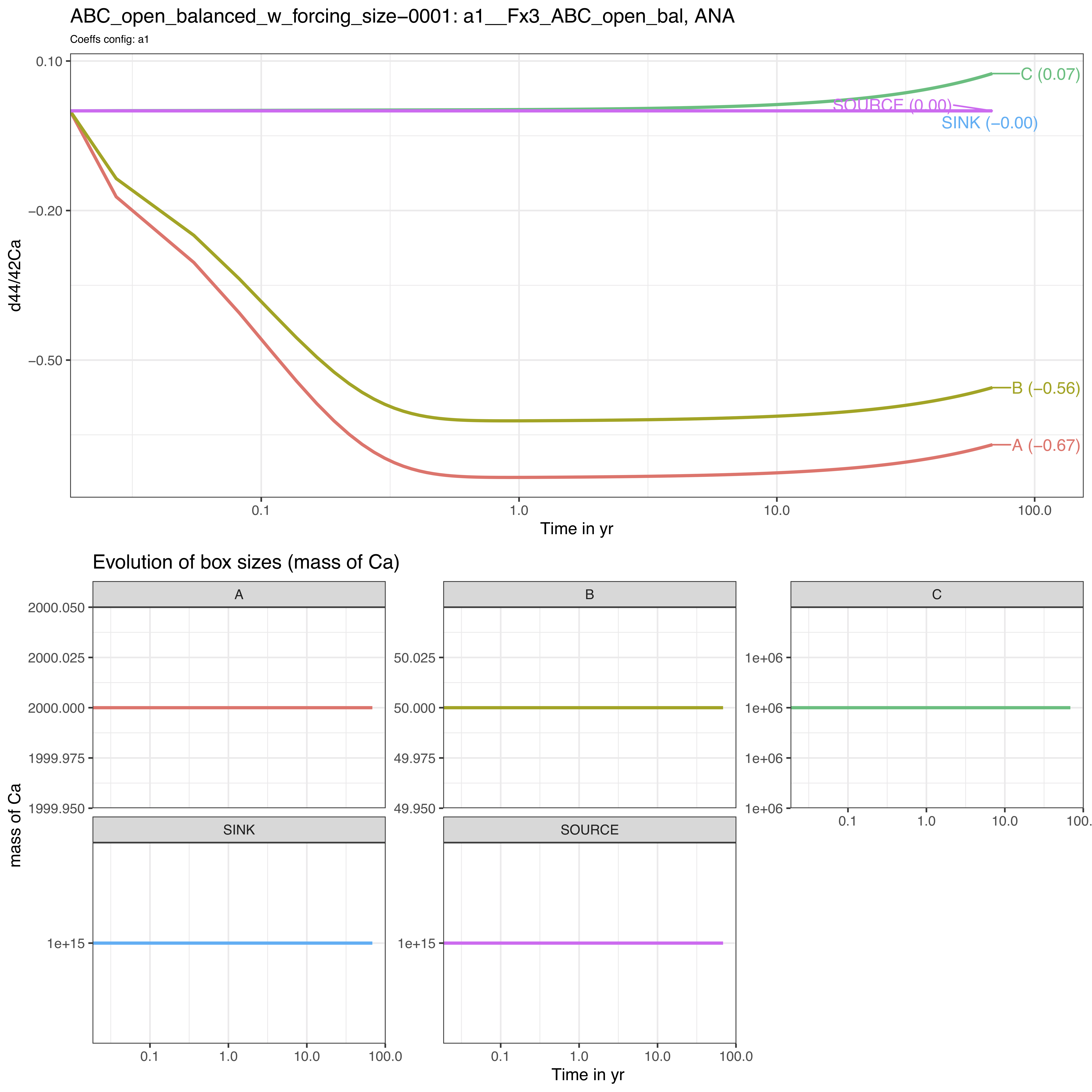
We observe that the system behaves very differently.

The steady-state is not reached over the run duration (25000 days).

The box C reacts very slowly in comparison to boxes A and C, as its size is several order of magnitudes higher than boxes A and C (1 000 000 against 2000 and 50).

The box C drives the dynamics of the system on the long-term.

4 - Run_isobxr: tutorial

Théo Tacail

1 Prepare tutorial

2 Ex. 1: {ABC}, closed, balanced

2.1 System definition

2.2 Run the model

2.3 Run outputs

2.3.1 System diagrams

2.3.2 Plots

2.3.3 Optional data outputs

3 Ex. 2: {ABC}, closed, unbalanced

3.1 System definition

3.2 Run the model

3.3 Run outputs

3.3.1 System diagrams

3.3.2 Plots

3.3.3 Optional data outputs

4 Ex. 3: {ABC}, open, balanced

4.1 System definition

4.2 Run the model

4.3 Run outputs

4.3.1 System diagrams

4.3.2 Plots

5 Ex. 4: Add forcing parameters

5.1 Forcing deltas

5.2 Forcing box sizes